Appetizer
08-30-2025
Did you ever wonder how to optimally pack parcels, serving customers with various subscription sizes while avoiding a dangerous goods shipping penalty fee? No? Well, me neither. Let’s investigate how its done anyways! Stay with me, its worth it: we will reduce shipping cost by 55% just by intelligently exploiting the degressive cost-per-weight structure in today’s CEP sector and reduce our cost to serve by up to 20%. We will rediscover the knapsack problem along the way and prove optimal bin allocation alone yields lower-than-industry cost to serve. Enough for the hook. Let’s do it!
Table of contents
- Introduction
- Case study: minimizing The Oater’s cost to serve
- Methodology
- Results and discussion
- Conclusion
- Code
Introduction
The German logistics market had a total volume of €327 billion in 2023. This makes logistics the third largest economic sector in Germany after the automotive industry and trade. Approximately half of the total volume originates from internal company’s logistics. The other half is generated by dedicated package delivery, courier and transportation companies. Logistic services are divided into general cargo (traditional pallets, special transports) and the more standardized CEP sector (DSLV). The transportation companies’ CEP sector was reported to make up around 16% of the total revenue and thus generates a turnover of 27 billion euros, which is comparable to the German consumer electronics market (CEP). In 2023, the CEP sector delivered around 4.51 billion parcels in Germany. Approximately 50% of this in terms of revenue and number of shipments were delivered by Deutsche Post DHL Group, the world’s second-largest logistics company after FedEx (Transportation companies by size).
CEP
The term CEP is the abbreviation for “Courier, Express and Parcel Services”. It refers to postal and logistics companies that primarily transport consignments with comparatively low weight and volume - such as letters, small packages, documents or small items. These restrictions on dimensions and weight allow a high degree of standardisation in processing. As a result, the handling and sorting of the objects to be transported can be easily (partially) automated. In this way, consignments can be transported in a short time and with high efficiency. (DHL dictionary)
The CEP sector is highly automated, which makes it cost-efficient. Consumers benefit significantly from low costs, as CEP enables access to a wide range of products offered on B2B and B2C marketplaces. However, since differentiation among CEP providers is limited, carriers create artificial service tiers to enforce differentiation and capture better prices. For example, logistics providers offer up to seven distinct classes within the \(0–31.5 \text{kg}\) range, with cost per weight decreasing as total weight increases. This results in a discrete buy-in to a given weight class, with any additional weight up to the class limit being effectively free, until the next buy-in at the following weight class becomes necessary. Other differenciation features might be present such as dangerous goods shipping fee, girth limits and more. This work exploits these discrete and predefined class features to allocate goods in an optimal way minimizing the cost to serve.
Comparing a standardized shopping cart with an allocation-optimized shopping cart we reduce the carrier cost by up to 55%. To understand the degrees of freedom that are available for optimization we will briefly introduce the CEP and warehousing sector as well as The Oater’s product portfolio and delivery frequencies.
CEP sector - weight and girth length matter
In order for the CEP sector to operate in a particularly cost-efficient manner and offer low prices to consumers, it is highly standardized with parcels meeting strict criteria in order to be processed as CEP. Three criterias are always applicable:
- weight with most transportation companies delivering parcels up to 31.5kg (70lbs)
- girth with most transportation companies limiting girth + length between 3000 and 4000 mm
- dangerous goods are generally excluded from CEP transportation unless they are transported in limited quantity, smallest quantities or products that are individually exempt from the dangerous goods transportatin prohibition according to ADR 3.3, 3.4, 3.5 (see (ADR)
Girth / Girth + length
The girth is the maximum permitted parcel size. It is calculated as: girth = 2 x (height + width). Most companies use girth + length = 2 x (height + width) + length to determine the maximum parcel size (DHL Dictionary, DPD FAQ).
To ensure that the delivery can be carried out particularly quickly (especially without material handling equipment such as forklifts), packages must not exceed a maximum permissible weight. This varies from provider to provider, but is centered around around 31.5 kg. Girth + length ensures that apart from weight a certain “density” maintained. Space is expensive and girth + length ensures a lower bar on what might be a cheap parcel in terms of wight but taking up overproportionally large space in the transportation vehicles. The product portfolio that is subject to optimization is dense enough such that we omit the girth + length constraint. Dangerous goods are less an economic category than a legal one, defined by the agreement of September 30, 1957 concerning the International Carriage of Dangerous Goods by Road (ADR) from 1957 ensuring safe transportation. This agreement categorizes goods for road transport, defines warning and safety instructions and lists exceptions. Exceptions include:
- simplified transport of certain dangerous goods when carried in small quantities as part of a company’s ancillary activities (e.g., maintenance, repair, construction) according to Special Provision SV1 (ADR 3.3)
- limited quantities (LQ) allows exemptions from most ADR provisions when dangerous goods are packaged in very small quantities per inner and outer packaging (ADR 3.2)
- Lithium-ion batteries in different sizes according to total capacity, cell size with respect to packaging, and prior certification
- blood and tissue samples when transported in specific packaging and quantity The cleaning detergent in The Oater’s product portfolio is subject to the LQ-regulation and may thus be shipped in one liter units when a fee is paid to the carrier insuring the carrier against leakage that might cause loss and damage to other goods in the cargo haul.
Warehouse - every pick matters
While a carrier only provides transportation services and thus assumes that the company itself is in physical possession of the outbound goods, this is not always the case. Most retailers and manufacturers rely on yet another third party that provides storage space. Typically this party is referred to as warehouse provider. Optionally, the warehouse provider also provides order administration and packaging. In case the whole value chain is fullfilled via a third party, one refers to this as third-party-logistics (3PL), adressing carrier, warehouse and packaging
Warehouses hold space for incoming goods, storage, a dedicated picking system, a packing area and a freight forwarding area where parcels are handed over to the carrier. Consequently service providers typically attribute cost for the administration and processing of incoming goods (usually on paletts), the administration of orders, the pick from a palett, the packing into carton and the placing into cargo space. A pick is associated with one product category, regardless of the quantity of the product. The occupied warehouse space is charged on a daily rate.
It makes sense to bundle consecutive orders per customer in order to save on additional picking costs (picking two pieces of the same type at the same time is cheaper than picking the same piece at two times). Apart from that, the strict billing system, in which every single step is charged individually, leaves little room for cost optimization shifting focus from warehouse back to CEP provider. The largest savings are generated by levelizing the administration fee over more liters in the monthly subscription.
3PL
Third-Party Logistics (3PL) refers to a business model in which a company outsources its logistics processes to an external service provider, a “third party”, regardless of the part of the logistics provided. Typically logistic processes are divided into warehousing/storage, usually including the control of incoming and outgoing goods (administration, picking, packing, truck loading) while another party takes care of transportation. While some companies offer a full-service other companies only provide one or some of the mentioned services. (Red stag fulfillment)
Case study: minimizing The Oater’s cost to serve
The Oater product portfolio
The Oater produces The Oater Barista, an automated oat drink production machine. The machine mixes water, an oat-based dry mix, as well as canola oil yielding oat drink through fermentation. After production, The Oater Barista doses a cleaning detergent into the reactor. The Oater Barista’s batch production is patented. Interested? Read on here.
Dry mix, oil and cleaning detergent are sent to the customer on a monthly basis. The quantities depend on the subscription volume (\(a\)) chosen by the customer. Dry mix, oil, and cleaning detergent are only available in a single container size. The cleaning detergent’s container size is limited by ADR section 3.2.
The The Oater Barista machine uses exactly one dry mix pouch, \(\frac{1}{5}\) of an oil bottle and \(\frac{1}{9}\) of a cleaning detergent bottle to produce 4.5 liters of oat drink in a single production cycle. Consequently
- one pouch of dry mix is sufficient to produce 4.5 liters of oat drink
- one bottle of oil is sufficient to produce 22.5 liters of oat drink
- one bottle of cleaning detergent is sufficient to produce 40.5 liters of oat drink.
Note that not only the net weight of the consumable goods must be considered, but also the gross weight, which includes the paper pouch and (glass/plastic) bottle. In addition, shipments can only be made in complete quantities.
Methodology
Given a known customer’s subscription size (\(a\)) and a known shipping-cost-to-weight vector (\(V\)) and known dangerous goods penalty (\(\Phi\)), as well known costs for warehousing and carrier we want to find the packing rule that yields minimal cost to serve the customer. We assume that girth size is never a limiting factor due to the high density of the individual products. Instead of minimizing only transportation cost we will look at the cost to serve. We will refer to this as the shipping-cost-problem.
As a heuristic we place all bottles of cleaning detergent in a single parcel so that the penalty is only paid once. However, the different weight categories of dry mix, oil and cleaning detergent indicate that it may no longer be possible to make optimal use of the shipping weight, as the weight class of the cleaning detergent is no longer available or other parcels. Furthermore, the degressive cost structure of shipping costs might make it more attractive to pack two medium-weight packages than one very heavy and one light package. It renders obvious that there is no simple instruction that guarantees minimal cost. We will therefore proceed to mathematical optimization.
Mathematical optimization
Mathematical optimization, also known as mathematical programming is the art of selecting of the best solution, given a set of conditions that have to be fullfilled exactely (equality constraints) as well as a set of conditions that have to be fullfilled but may vary in a given range (inequality constraints). The equation that defines how a good solution is measured is called cost function. The nature of the variables involved in the cost function and in the constraints then define the problem category and thus lastly solution approach. Mathematical programming is used everywhere, from routing problems, AI training to advanced process control and has equal origins in the chemical engineering community as well as in operations research. The interested reader is directed to my former Professor Stratos Pistikopoulos who taught me optimization (see Parametric) as well as his dear collegues in the field such as Professor Alexander Mitsos (see SVT). Furthermore I suggest reading articles in CACE, and EJOR, both great journals to follow and inspire how today’s engineering problems are solved via optimization.
Cost of goods
We base the solution algorithm on the price per liter of produced oat drink and define a known monthly subscription model size \(a\). The known number of oat packs \(N_T\), oil bottles \(N_O\) and cleaning agent bottles \(N_R\) are consequently given by ceiling to the largest natural number that statisfies \(a\) and are stored in \(N\):
- \[N_T = \left\lceil a/4.5 \right\rceil\]
- \[N_O = \left\lceil a/22.5 \right\rceil\]
- \[N_R = \left\lceil a/40.5 \right\rceil\]
where \(N = [N_T \quad N_O \quad N_R] \in \mathbb{N^3}\). Consequently the number of species subject to optimization is \(N_S=3\). Each item has a known weight \(w = [w_T, w_O, w_R]^\top\) in kilo gram, and a known cost-per-piece \(c = [c_T, c_O, c_R]^\top\) in Euro.
Carrier cost
Carrier cost can be obtained by the multiplication of a cost-per-weight vector with a distribution matrix holding the content of each parcel.
Shipping cost vector
The shipping cost vector \(V\) holds the price-per-parcel (\(SC\)) within the associated shipping weight class (\(SW\)). We remove 1.5 kg from each parcel to account for carton and filling weight.
\[V = \begin{bmatrix} SC & SW \\ \end{bmatrix}^\top = \begin{bmatrix} 0 & 0 \\ 3.62 & 1.5 \\ 4.17 & 3.5 \\ 4.83 & 8.5 \\ 6.30 & 13.5 \\ 6.85 & 18.5 \\ 7.02 & 23.5 \\ 7.29 & 30 \end{bmatrix}^\top\]For better understanding figure 1 visualizes the piecewise linear nature of \(V\), mapping parcel cost to weight. The blue curve plots the parcel cost over the admissable parcel weight. Notice that a flat slope indicates a good weight to cost ratio. The cost per weight are steadily decreasing, making heavy parcels most efficient.
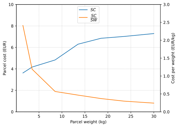
The length of \(V\) is the number of different weight/cost categories provided by the CEP, here \(N_V= 8\), as we include the null-weight/cost as a convenient way to attribute zero cost associated with an empty, never packed parcel. Last we define the dangerous goods shipping cost penalty as \(\phi=3.5\) as a one-time fee added to each parcel that contains \(\geq1\) cleaning detergent bottles.
Parcel content and weight
In oder to calculate the weight efficiently we introduce the distribution matrix \(D \in [N_S, N_T+N_O+N_R=N_L]\) holding the number of items per species per parcel. As an upper bound for the number of parcels necessary to ship all items we conveniently use the sum of all individual items. Additionally, we introduce the cost category matrix \(C \in [N_V, N_L]\) a zero-matrix consisting of zeros exept for the respective cost category of each parcel denoted with a \(1\). We lastly define a penalty vector \(\Phi \in [N_L]\) holding zeros for each parcel except for ones for the parcel that hold \(\geq1\) cleaning detergent bottles. Consequently \(\Phi\) is a binary optimization variable.
Warehouse cost
Warehouse cost assume that each subscription triggers only one monthly “warehouse run”, even if the total shopping cart is then packed in more than one parcel. For ease of understanding we separate the warehouse cost \(c_{\text{warehouse}}\):
\[\begin{align} c_{\text{warehouse}} &= c_{\text{pick}}+c_{\text{parcel}} \\ c_{\text{pick}} &= c_A + c_P \cdot N_S \\ c_{\text{parcel}} &= c_p \cdot \sum^P \sum^C C_{c,p} \end{align}\]where \(c_A\) is the per-subscription order administration fee and \(c_P\) is the per-pick fee. Both fees are known and warehouse provider dependent. \(c_{\text{parcel}}\) is a warehouse provider dependent cost associated with carton, filling and freight farwarding of each parcel and is thus multiplied with the number of parcels that servce the monthly subscription. To conveniently grasp the number of parcels we rely on \(C\).
Cost function
The cost to serve (\(CTS\)) of one liter of oat-drink is the sum of the cost of goods \(CG\), the carrier cost \(CC\) and the warehouse cost \(WC\):
\[CTS(V,\phi) = \min_{D,\Phi,C} \frac{1}{a} (CG + CC + WC)\]and are a function of the shipping-cost vector and the penalty fee. We assume \(N\) not to be subject to optimization. Inserting the discrete terms for each associated cost the cost function becomes
\[CTS(V,\phi) = \min_{D,\Phi,C} \frac{1}{a} (N \cdot c + \sum^C\sum^P SC_c \cdot C_{c,p} + \sum^P \phi \cdot \Phi_p + c_A + c_P \cdot N_S + c_p \cdot \sum^C \sum^P C_{c,p})\]We optimize for the lowest possible cost to serve and calculate the fractions of \(CG, CC, WC\) in post-processing.
Shipping cost problem
The shipping cost problem is given as
\[\begin{align} CTS(V,\phi) &= \min_{D,\Phi,C} \frac{1}{a} (N \cdot c + \sum^C\sum^P SC_c \cdot C_{c,p} + \sum^P \phi \cdot \Phi_p + c_A + c_P \cdot N_S + c_p \cdot \sum^C \sum^P C_{c,p}) \tag{a}\\ \text{s. t.} \quad \sum^P D_{s,p} &= N_s \quad \forall s \in S \tag{b}\\ \sum^C C_{c,p} &= 1 \quad \forall p \in P \tag{c}\\ \sum^S D_{s,p} \cdot w_s &\leq SW_1 \cdot C_{1,p} + SW_{N_V} \cdot (1 - C_{1,p}) \quad \forall p \in P \tag{d}\\ SW_{c-1} \cdot C_{c,p} &\leq \sum^S D_{s,p} \cdot w_s \quad \forall p \in P, c \in C \setminus [1] \tag{e}\\ \sum^S D_{s,p} \cdot w_s &\leq SW_c \cdot C_{c,p} + SW_{N_V} \cdot (1 - C_{c,p}) \quad \forall p \in P, c \in C \setminus [1] \tag{f}\\ D_{N_S,p} &\leq N_R \cdot \Phi_p \quad \forall p \in P \tag{g} \end{align}\]Equation (b) guarantees that all items are shipped to the customer and equation (c) ensures only one weight category may be selected. Equation (d) serves a double purpose: first it provides a null-cost category, representing an empty and thus unshipped parcel. Additionally, in case the parcel is not empty, the maximum admissible parcel weight is set as an upper bound. Equation (e,f) finally select the correct cost category. Notice that the RHS of equation (e) is the LHS of equation (f). What could be written as a single line in math notation has to be split apart first and then handed to the optimizer. Lastly equation (g) sets the penalty pin in case cleaning detergent is in the parcel. Notice that the cost function then conveniently sums over all elements in \(\Phi\).
Solution strategy
The shipping cost problem holds linear terms as well as integer decision variables only. While \(D\) holds an integer decision variables; \(C, \Phi\) hold binary decision variables. Thus, the shipping cost problem is an integer programming problem and can be solved with standard IP solvers. The problem was solved with Gurobi Optimizer version 10.0.3 on an Apple M3 Pro SoC running 12 threads with 18GB RAM in Visual Studio version 1.101.2. The model consists of 1140 integer decision variables of which 855 are binaries for a subscription size of 320 liters and solved to optimality in 0.04 seconds for generation and 0.17 seconds for optimization. Since \(SW \ll 1e+5\) in \(D \cdot w \leq SW \cdot C\) in equation (f), we omitted setting Gurobis’ IntegralityFocus parameter.
Integrality focus
Since \(C\) is binary, Gurobi assumes values for binaries that are as large as \(10^{-5}\) as \(0\). In case \(SW \gg 10^5\), this would not effectively enforce the intended relationship that \(D\) must be zero if \(C\) is zero. To circumvent the effect known as trickle flow Gurobi has the option to set the IntegralityFocus parameter. This makes Gurobi work really hard to make sure zeros are actual zeros by assuming only variables as large as \(10^{-9}\) as \(0\) (see IntegralityFocus).
For \(a=1000\), the model was solved to optimality in 0.10 seconds for generation and 0.83 seconds for optimization. This is remarkably fast for a model holding \(|C| \approx 10^3\) binaries. Consequently we will not investigate runtime improvement through problem reformulation. Gurobi does an excellent job at presolving and facilitating the problem before optimization.
More on runtime will come soon
I will add a follow-up investiagation on solver and modeling language specific runtime, solving the shipping cost problem in Julia using JuMP, ORTools’ CP-SAT and HiGHS. Come back later. Note that my publication on flexibility already investigated the effects of omitting big-M constraints using SOS1 constraints instead on model generation and model optimization time.
Notice shipping cost optimization extends bin packing, itself an extension of the NP-hard knapsack problem. The classical knapsack problem (see Knapsack 1, Knapsack 2) asks how to select a subset of items, each with a value and a weight, such that the total weight does not exceed a given capacity while maximizing the total value. This problem is already NP-hard, as the feasible solution space grows combinatorially with the number of items. A natural extension is the bin packing problem (see Wikipedia), which shifts the focus from maximizing value to minimizing the number of bins required to hold all items, given fixed bin capacities. Its defining feature is the binary big-M style decision whether an item is placed in a particular bin. The shipping cost problem follows the same logic (see shipping cost problem’s equations d, e, f). Like bin packing, it uses binary allocation constraints, but it extends the model by introducing discrete cost classes for bins. Instead of minimizing only the number of bins, the objective is to minimize cost to serve by choosing not just how many bins are used but also which type of bins are selected. Thus, while inheriting the NP-hard complexity of knapsack and bin packing, the added dimension of discrete bin costs renders my problem even more challenging.
Results and discussion
Figure 2 shows the cost by categoy and their share of the total cost to serve. The horizontal axis of the figure represents the monthly subscription size. The cost to serve \(CTS\), warehouse cost \(CW\) and carrier cost \(CC\) are represented by solid lines and represented on the left y-axis. The proportions of the cost of goods \(\frac{CG}{CTS}\), warehouse cost \(\frac{CW}{CTS}\) and carrier cost \(\frac{CC}{CTS}\) are represented by dashed lines and represented on the right y-axis.
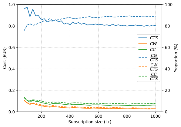
The cost to serve approach a steady state starting from monthly subscription sizes of around 500 liters and more. The per-liter cost of goods are almost invariant with only minor effects through ceiling. Thus when a steady-state \(CTS\) is reached, this can only be achieved through a steady state in warehouse and carrier costs. The overall \(CTS\) savings are \(18.3\%\) when comparing the most unfortunate subscription size of 100 liters per month with the best possible subsciption size of 920 liters per month.
To further investigate this issue figure 3 shows the relative savings for warehouse cost (\(\eta_W\)) and carrier cost (\(\eta_C\)) compared against the \(a=80\) base case as this reflects the smallest available subscription size at The Oater. The findings from figure 2 are verified. Also the relative savings both for warehouse and carrier cost approach a near steady-state/saturation effect starting from around 500 liters per month.
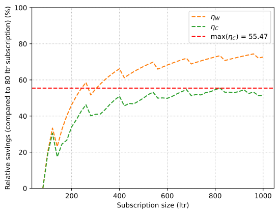
Just by optimally bundeling goods we achieve carrier cost savings of 55.5%. We save even more on warehouse expenses with savings of up to 74.4%. However, since the carrier cost are higher in absolut terms, carrier savings are more valuable to minimize cost to serve.
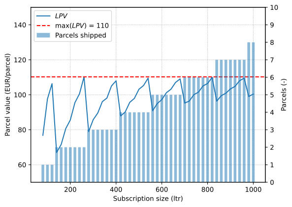
Lastly, let’s investigate the effect of shipping cost optimization from a different angle. Figure 4 shows the levelized per-parcel value (\(LPV = \dfrac{CTS \cdot a}{|\text{parcels}|}\)). As parcels are filled, \(LPV\) increases in a predictable manner. Once an additional box must be introduced, \(LPV\) drops sharply, which in turn reduces the overall cost efficiency of the carrier. This apparent loss can be mitigated by reverting to a smaller parcel category, defined by lower weight and cost, which dampens the decline in savings. The observed reductions in \(LPV\) align precisely with corresponding declines in \(\eta_W\) and \(\eta_C\) (see figure 3), although the latter effect is less pronounced.
Conclusion
A strongly negative effect of the dangerous goods surcharge is not apparent. Looking at \(\Phi\), we observe that dangerous goods are only divided into two packages for subscription sizes of 940 liters or more. This only happens because dangerous goods required to serve subscription sizes of 940 liters and more exceed the weight limit for a single parcel. Bundling all cleaning detergent bottles into a single parcel indicates that the weight of a cleaning detergent bottle does not offer sufficient flexibility to achieve savings per weight through the clever filling of a package, despite the dangerous goods surcharge. This may be due to the fact that a cleaning detergent bottle weighs about twice as much as dry mix, whose quantity surpasses the cleaning detergent’s quantity (\(N_T \approx 10 \cdot N_R\), \(w_T \approx 0.5 \cdot w_R\)). Instead of utilizing a bottle of cleaning detergent to fill up free weight, two dry mixes are utilized instead.
In summary: optimal bin packing reduces the cost to serve by up to 20% with savings in carrier costs of up to 55%. No particular pressure of the dangerous goods penalty on the bin packing was observed. The optimal solution coincides with the simple heuristic of placing all cleaning detergent bottles into a single package. Efficiency losses arise primarily when an additional parcel must be added to fulfill the subscription, thereby reducing the value per parcel. These losses are partially mitigated by downsizing to smaller and thus cheaper parcels but still translate into higher carrier costs. Despite this, The Oater realizes substantial savings through optimized shipping, directly improving margin. Moreover, on-premise oat drink is largely a low-margin FMCG, where decreasing the cost to serve at higher volumes is more effective than increasing the price per liter for the customer.
The case study showed combined warehouse and carrier costs of about 20% for small and as low as 10% for large subscriptions, excluding return shipments. In comparison to industry standards The Oater is operating at the lower end through optimized goods allocation (see The geography of transport systems, Amazon’s logistics costs, Business insider).
Code
Want to get started on your own? Try out differenct cost vectors and penalties? In depth analyse the data? Clone my repository here. I provided the optimization as well as the visualization script as well as the results in a concise csv file. Enjoy.